Background

Using devices such as Jawbone Up, Nike FuelBand, and Fitbit it is now possible to collect a large amount of data about personal activity relatively inexpensively. These type of devices are part of the quantified self movement - a group of enthusiasts who take measurements about themselves regularly to improve their health, to find patterns in their behavior, or because they are tech geeks. More information, including the data for this project, is available from the website here: http://groupware.les.inf.puc-rio.br/har (see the section on the Weight Lifting Exercise Dataset).

Data Load and Preprocessing

Training and testing datasets (containing 19622 and 20 observations of 160 variables, respectively) were loaded in the working directory.
First, columns with more than 20% of NAs were removed from both training and testing sets. Next, the original training dataset was split into two parts, a training (70% of the original training set) and a validation set (30% of the original training set) for cross-validation. That is, a predictive model has been built on the new training set, and evaluated on the validation data set. The first column of the every data set is simply the index, and has been removed as it is not a predictor variable. In addition, an effort was made to remove near zero variance predictors, though none was identified as such and, in turn, no additional column was removed. Lastly, all data sets were standardizing using caret’s preProcess function.

# Download data sets in the working directory
fileUrl1 <- "https://d396qusza40orc.cloudfront.net/predmachlearn/pml-training.csv"
fileUrl2 <- "https://d396qusza40orc.cloudfront.net/predmachlearn/pml-testing.csv"
download.file(fileUrl1,destfile="pml-training.csv")
download.file(fileUrl2,destfile="pml-testing.csv")

library(caret)

## Loading required package: lattice
## Loading required package: ggplot2

set.seed(12345)

# Load data sets 
training0 <- read.csv("pml-training.csv",header = TRUE,
                      na.strings = c("NA",""))
test0 <- read.csv("pml-testing.csv",header = TRUE,
                  na.strings = c("NA",""))

# Remove columns that contain NAs more than 20% of total observation
training0 <- training0[, colSums(is.na(training0)) < 0.2*nrow(training0)]
test0 <- test0[, colSums(is.na(test0)) < 0.2*nrow(test0)]

# Split the training set into two parts, training and validation sets
inTrain <- createDataPartition(y=training0$classe, p=0.7, list=FALSE)
training <- training0[inTrain,-1]
validation <- training0[-inTrain,-1]
test <- test0[,-1] 
# The first column (X) with index was removed from all data sets

# Identification of near zero variance predictors
nzv <- nearZeroVar(training,saveMetrics = TRUE)
summary(nzv$zeroVar)

##    Mode   FALSE    NA's 
## logical      59       0

# Standardizing using preProcess function
preObj <- preProcess(training[,-59],method=c("center","scale"))
training <- predict(preObj,training)
validation <- predict(preObj,validation)
test <- predict(preObj,test)

Building a Predictive Model

First, the predictive model was built using a Random Forest classification method with 3-fold cross-validation for the training set. As shown below, the random forest classification model has 500 trees, #No. of variables tried at each split is 41, and OOB estimate of error rate is 0.09%, which is excellent.

library(caret); library(randomForest)

## randomForest 4.6-12
## Type rfNews() to see new features/changes/bug fixes.
## 
## Attaching package: 'randomForest'
## 
## The following object is masked from 'package:ggplot2':
## 
##     margin

# Build a model using Random Forest and resampling for cross validation
modFit.rf <- train(classe~., method="rf", data=training, 
             trControl = trainControl(method="cv"),number=3)

modFit.rf$finalModel

## 
## Call:
##  randomForest(x = x, y = y, mtry = param$mtry, number = 3) 
##                Type of random forest: classification
##                      Number of trees: 500
## No. of variables tried at each split: 41
## 
##         OOB estimate of  error rate: 0.09%
## Confusion matrix:
##      A    B    C    D    E  class.error
## A 3905    1    0    0    0 0.0002560164
## B    1 2657    0    0    0 0.0003762227
## C    0    3 2391    2    0 0.0020868114
## D    0    0    1 2249    2 0.0013321492
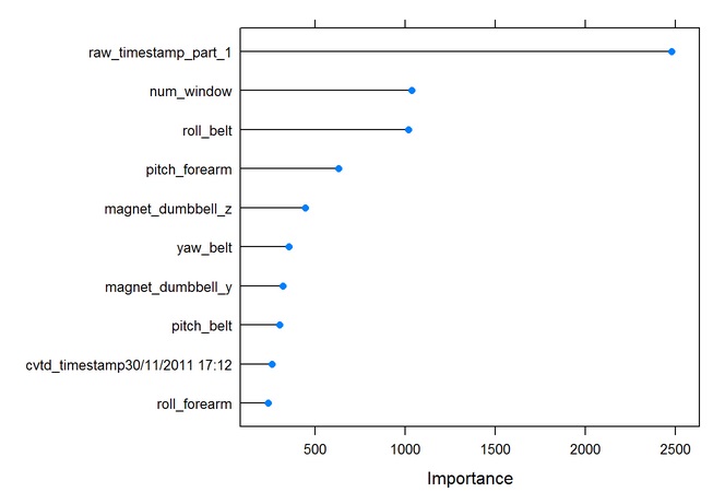
## E    0    0    0    2 2523 0.0007920792

# Plot the importance of predictor variables
rfImp <- varImp(modFit.rf,scale=FALSE)
plot(rfImp, top=10)

Prediction of the validation set and Out of sample error

Random Forest model accuracy of the prediction upon the validation set is 0.9997 or 99.97%. In other words, Out of sample error is 0.0003 or 0.03%.

# Predict the validation set
pred.rf <- predict(modFit.rf, newdata=validation)
confusionMatrix(pred.rf, validation$classe)

## Confusion Matrix and Statistics
## 
##           Reference
## Prediction    A    B    C    D    E
##          A 1674    0    0    0    0
##          B    0 1139    1    0    0
##          C    0    0 1025    0    0
##          D    0    0    0  964    1
##          E    0    0    0    0 1081
## 
## Overall Statistics
##                                      
##                Accuracy : 0.9997     
##                  95% CI : (0.9988, 1)
##     No Information Rate : 0.2845     
##     P-Value [Acc > NIR] : < 2.2e-16  
##                                      
##                   Kappa : 0.9996     
##  Mcnemar's Test P-Value : NA         
## 
## Statistics by Class:
## 
##                      Class: A Class: B Class: C Class: D Class: E
## Sensitivity            1.0000   1.0000   0.9990   1.0000   0.9991
## Specificity            1.0000   0.9998   1.0000   0.9998   1.0000
## Pos Pred Value         1.0000   0.9991   1.0000   0.9990   1.0000
## Neg Pred Value         1.0000   1.0000   0.9998   1.0000   0.9998
## Prevalence             0.2845   0.1935   0.1743   0.1638   0.1839
## Detection Rate         0.2845   0.1935   0.1742   0.1638   0.1837
## Detection Prevalence   0.2845   0.1937   0.1742   0.1640   0.1837
## Balanced Accuracy      1.0000   0.9999   0.9995   0.9999   0.9995

The current Random Forest model appears to be almost perfect, leaving little room for improvement. Thus, it was chosen as the final predictive model and no additional effort was made to further fine-tune it.

Prediction of the test set

Finally, the Random Forest model was applied to predict 20 different test cases, which resulted in 100% accuracy.

#Predict the test set using the Random Forest model
predRF_Test <- predict(modFit.rf, newdata=test)
predRF_Test

##  [1] B A B A A E D B A A B C B A E E A B B B
## Levels: A B C D E

Conclusion

The Random Forest classification model in combination with a couple of simple data preprocessing procedures (such as removing irrelevant data columns and standardizing) is turned out to be a great approach to predict the manner in which people did the exercise, using the given data from accelerometers on the belt, forearm, arm, and dumbell of participants.